Quickstart

We take one district from a measured prevalence to a plotted trajectory.

One scenario

A Scenario holds one candidate campaign, the setting as it stands and the intervention that switches on at the campaign, where EirTarget(0.45, "prevalence") tells run_scenarios that 0.45 is a measured prevalence rather than an EIR, so it is inverted into a baseline EIR before the emulator runs.

from estimint import Scenario, EirTarget, run_scenarios

pbo = Scenario(
    name="PBO switch",
    res_use=0.30,          # pyrethroid resistance
    Q0=0.85,               # share of bites taken on humans
    phi=0.80,              # share of bites taken in bed
    seasonal=0.0,          # 0 perennial, 1 strongly seasonal
    irs=0.0,               # current IRS coverage
    eir_target=EirTarget(0.45, "prevalence"),

    py_only=0.70,          # current nets: pyrethroid-only at 70% coverage

    itn_future=0.70,       # the campaign: same coverage...
    net_type_future="pyrethroid_pbo",   # ...different net
)

Note that itn_future=0.70 has to be set explicitly, since a Scenario that leaves its _future fields out withdraws the intervention at the campaign rather than keeping the nets in place.

Run the scenario

run_scenarios converts each net mix and resistance level to dn0, inverts each measured prevalence to a baseline EIR, and calls the emulator. It returns one row per scenario.

results = run_scenarios([pbo])

results.drop(columns=["prevalence", "cases"]).T

	0
name	PBO switch
input_mode	prevalence
net	py_only
net_future	pyrethroid_pbo
dn0_use	0.311
itn_use	0.7
irs_use	0.0
dn0_future	0.48495
itn_future	0.7
irs_future	0.0
routine	0.0
lsm	0.0
seasonal	0.0
eir_baseline	31.960129
mosquito_delta	0.0
eir_final	31.960129
hbr_baseline	NaN
hbr_new	NaN
prev_y9	0.456028
prev_endline	0.470118
cases_endline	2.412444

dn0_use is the lethality of the nets on the ground today, and dn0_future that of the PBO nets replacing them. eir_baseline is the transmission intensity implied by that prevalence, in infectious bites per person per year. prev_y9 is prevalence at the campaign, prev_endline three years after it, and cases_endline the clinical case rate there.

hbr_baseline and hbr_new are NaN, because they are only computed when a prevalence input is paired with a non-zero mosquito_delta.

The trajectory

The two columns dropped from the table, prevalence and cases, hold the trajectories, each cell a 157-element NumPy array. The elements are 14-day windows starting at day 2190, with the campaign at day 3285.

import numpy as np

prev = results.loc[0, "prevalence"]

abs_t = 2190 + 14 * np.arange(len(prev))   # day of each 14-day window
years = (abs_t - 3285) / 365               # years from the campaign

print(prev.shape, years[0].round(2), years[-1].round(2))

(157,) -3.0 2.98

fig, ax = plt.subplots(figsize=(7, 4))

ax.plot(years, prev, color="#00d4aa", lw=2)
ax.axvline(0, color="#8b93a3", ls="--", lw=1, alpha=0.7)

ax.set_xlabel("Years from the campaign")
ax.set_ylabel("Under-5 prevalence")
ax.set_ylim(0, None)

plt.show()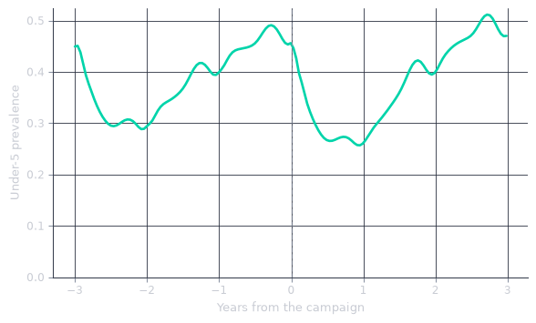

A green line chart of prevalence against years from the campaign. Prevalence wanders between about 0.29 and 0.50 over the three years before the campaign and reaches 0.46 at it, then drops sharply to about 0.26 a year after the campaign before climbing back to about 0.47 by the end of the third year. — Under-5 prevalence for a switch to pyrethroid-PBO nets at 0.70 coverage, in a setting with resistance 0.30 and a measured prevalence of 0.45. The grey dashed line marks the campaign.

The green line reaches its minimum about a year past the grey dashed campaign line, then climbs back over the remaining two years to finish close to where it started, because the insecticide on a net decays across the three years it spends in the field. The endline value on its own understates the campaign.

EirTarget pins prevalence at the campaign, where prev_y9 comes out at 0.456 against the 0.45 that was measured, and everything left of the dashed line is the emulator’s own history of the setting under the nets already in place. The three years before the campaign are not flat.

One scenario

Run the scenario

The trajectory

See also