MINTverse runs in two stages because the emulator takes an EIR and a user almost never has one. The first stage inverts what was measured, a parasite prevalence or a human biting rate, into the EIR that would sustain it. The second stage runs the campaign forward from that EIR.
Stage one is estiMINT, three gradient-boosted trees and a curve fit, cheap and deterministic, returning the equilibrium at the decision point. It has no notion of time.
Stage two is stateMINT, a sequence model taking the twelve covariates, one row describing a setting and a campaign. It emits 157-step trajectories for prevalence and cases.
Between them sits calculate_dn0, a lookup against published resistance curves rather than a fitted model. It turns a net mix into the single lethality number both stages consume.
Using the pipeline
run_scenarios executes the diagram above, taking a list of Scenario objects, deriving dn0 from each net mix, applying any mosquito-density adjustment, and returning one row per scenario, with the trajectories stored as 157-element arrays in the prevalence and cases cells.
The low-level functions (calculate_dn0, load_xgb_model, run_xgb_model and Mamba2Regressor.from_pretrained) allow the pipeline to be entered part-way. Use them when EIR is already known from an entomological study, when the EIR itself is the required answer, or when you are sweeping a covariate that Scenario does not expose as a field.
What the emulator is emulating
stateMINT was trained on output from malariasimulation, the individual-based transmission model, and it reproduces that simulator to within its training error. It does so in milliseconds rather than minutes.
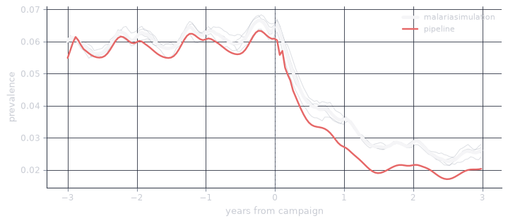
One held-out parameter set, under a campaign of nets and indoor spraying. The white line is malariasimulation, averaged over the individual stochastic runs drawn in grey. The red line is the pipeline, from a measured prevalence through estiMINT to stateMINT.
The red line follows the white one through the pre-campaign equilibrium and the drop when the campaign lands. It settles around a percentage point below the simulator in the final years. That residual is the emulator’s, and it is the size of error to expect. Every structural assumption malariasimulation makes is inherited whole, so a stateMINT trajectory answers what the simulator would have said rather than what a district will do. Accuracy and speed quantifies both halves of that error.
Domain limits
The emulator is only as good as the covariate space it saw in training. estiMINT is only as good as the prevalences it was fitted against.
estiMINT clamps its inputs to the calibrated domain, so that prev_y9 is clamped to \([0.005,\ 0.80]\) and hbr_y9 to \([5 \times 10^{3},\ 7 \times 10^{7}]\).
Clamping
Nothing is raised, logged, or flagged. A prevalence of 0.92 is clamped to 0.80 before the model sees it, and a prevalence of 0.001 is clamped to 0.005. The value that comes back looks like every other number the model returns.
Check your inputs against the bounds before you call. Treat an implausibly flat trajectory, or an EIR that does not change as prevalence is increased, as the signature of a clamped input rather than a finding.
Below 0.005 the prevalence-to-EIR relationship becomes near-vertical, and a vanishing change in prevalence maps to a large change in EIR, while above 0.80 the training library thins out, because settings that hyperendemic are rare in the parameter grid the simulations were drawn from. A scenario at the edge of the domain needs a sensitivity check. Perturb the inputs and check the conclusion holds.