import numpy as np
import pandas as pd
from estimint import run_scenarios, preload_models
from estimint.scenarios import Scenario, EirTarget

setting = dict(
    res_use=0.30, Q0=0.85, phi=0.80, seasonal=0.0, irs=0.0,
    py_only=0.70, routine=0.0,
    eir_target=EirTarget(0.45, "prevalence"),
)

scenarios = [
    Scenario(name="Withdraw", **setting),
    Scenario(name="Pyrethroid-only", itn_future=0.70,
             net_type_future="pyrethroid_only", **setting),
    Scenario(name="PBO", itn_future=0.70,
             net_type_future="pyrethroid_pbo", **setting),
    Scenario(name="Pyrrole", itn_future=0.70,
             net_type_future="pyrethroid_pyrrole", **setting),
    Scenario(name="PBO + IRS + LSM", itn_future=0.70,
             net_type_future="pyrethroid_pbo", irs_future=0.60, lsm=0.30, **setting),
]

res = run_scenarios(scenarios)Trajectories and cases
The list from A list of scenarios holds five campaigns run against one shared baseline. What comes back is five rows of scalars and five pairs of 157-step trajectories, and rebuilding it takes the same setting and the same five Scenario objects.
The time grid comes off the emulator’s own configuration rather than being hard-coded.
_, artifacts = preload_models()
cfg = artifacts["prevalence"].preprocessing_config

n_steps = cfg["n_steps"]
window = cfg["window_size"]

abs_t = cfg["model_start_day"] + window * np.arange(n_steps)
years = (abs_t - cfg["intervention_day"]) / 365
idx_y9 = int(np.argmin(np.abs(abs_t - cfg["intervention_day"])))

idx_y978Prevalence trajectories
fig, ax = plt.subplots(figsize=(7.6, 4.0))
for _, row in res.iterrows():
    ax.plot(years, row["prevalence"], lw=1.8, label=row["name"])
ax.axvline(0, color="#8b93a3", ls="--", lw=1, alpha=0.7)
ax.set_ylim(0, None)
ax.set_ylabel("Prevalence (under 5)")
ax.set_xlabel("Years since campaign")
ax.legend(ncol=2, fontsize=8)
plt.show()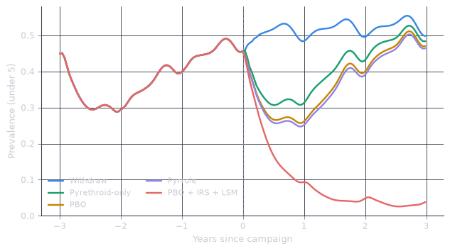
The five lines coincide to the left of the dashed line. That is the shared run-up under the pyrethroid-only nets already in place. After the campaign the three net scenarios reduce prevalence, reach a minimum roughly a year in, and converge towards one another as their insecticide decays, while withdrawal rises throughout and the combination scenario falls well below the other four and stays there. This is because IRS and larval source management do not decay on the same three-year clock a net does.
The three net scenarios end the horizon within about two prevalence points of each other. At their minimum they were separated by considerably more.
Clinical cases
The same five scenarios carry a second trajectory, clinical incidence, on the emulator’s own scale.
fig, ax = plt.subplots(figsize=(7.6, 4.0))
for _, row in res.iterrows():
    ax.plot(years, row["cases"], lw=1.8, label=row["name"])
ax.axvline(0, color="#8b93a3", ls="--", lw=1, alpha=0.7)
ax.set_ylim(0, None)
ax.set_ylabel("Clinical incidence")
ax.set_xlabel("Years since campaign")
ax.legend(ncol=2, fontsize=8)
plt.show()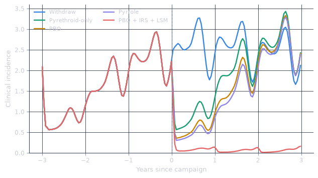
Incidence oscillates from one 14-day window to the next, far more than prevalence does, and by the right-hand edge the three net scenarios have converged into a band that overlaps withdrawal. This is because prevalence measures existing infection, while incidence records new episodes per window. Incidence inherits the window’s sampling noise.
res[["name", "cases_endline"]].sort_values("cases_endline").round(4)| name | cases_endline | |
|---|---|---|
| 4 | PBO + IRS + LSM | 0.1653 |
| 0 | Withdraw | 2.1272 |
| 3 | Pyrrole | 2.3899 |
| 2 | PBO | 2.4124 |
| 1 | Pyrethroid-only | 2.4331 |
Sorted on cases_endline alone, withdrawing the nets comes out ahead of every net scenario, an artefact of the column rather than something the campaigns did. The window is noisy, as the panel above shows. Clinical incidence is also not a monotone function of transmission, and the withdrawal scenario has spent three years at higher prevalence, so the simulator’s immunity dynamics carry that through into fewer clinical episodes per person late in the horizon.
A note on endline columns
prev_endline and cases_endline are single 14-day windows. They are cheap to sort on and they throw away the three years over which a campaign does its work. Integrate the trajectory instead.
Cases averted
Integrate cases from idx_y9, with the timestep expressed in years.
step_years = window / 365

totals = {}
for _, row in res.iterrows():
    totals[row["name"]] = float(np.trapezoid(row["cases"][idx_y9:], dx=step_years))

burden = pd.Series(totals, name="burden")

burden.round(3)
Withdraw 7.577
Pyrethroid-only 5.619
PBO 4.815
Pyrrole 4.548
PBO + IRS + LSM 0.295
Name: burden, dtype: float64cases is reported on the emulator’s own incidence scale, and because every scenario shares that scale, differences and percentages between them are meaningful without pinning the units. Taking withdrawal as the counterfactual gives the burden each campaign averts.
baseline = burden["Withdraw"]

averted = (
    pd.DataFrame(
        {
            "burden": burden,
            "averted": baseline - burden,
            "averted_pct": 100 * (baseline - burden) / baseline,
        }
    )
    .sort_values("averted", ascending=False)
    .rename_axis("campaign")
)

averted.round(2)| burden | averted | averted_pct | |
|---|---|---|---|
| campaign | |||
| PBO + IRS + LSM | 0.29 | 7.28 | 96.11 |
| Pyrrole | 4.55 | 3.03 | 39.98 |
| PBO | 4.81 | 2.76 | 36.46 |
| Pyrethroid-only | 5.62 | 1.96 | 25.85 |
| Withdraw | 7.58 | 0.00 | 0.00 |
bars = averted.drop(index="Withdraw").sort_values("averted_pct")

fig, ax = plt.subplots(figsize=(7.2, 3.4))
ax.barh(bars.index, bars["averted_pct"], height=0.55)
ax.set_axisbelow(True)
ax.set_xlabel("Clinical burden averted vs withdrawal (%)")
ax.set_xlim(0, 100)
plt.show()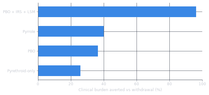
Integrated over the three years the nets are in the field, the three net scenarios are separated by around fourteen percentage points of averted burden. At endline they were separated by two prevalence points.
The ordering of the net scenarios follows dn0_future and nothing else, so it is only as good as the resistance level supplied, and at a resistance of 0.30 the pyrethroid-only and the pyrrole net are far apart, while at 0.0 they are much closer. A resistance estimate carries error. Re-run the scenarios across its plausible range to see how much of the ordering survives it.
See also
Exporting results gets these tables and trajectories out of Python. Nets and dn0 covers the resistance curves that set the ordering of the net scenarios. EIR, HBR, prevalence, and cases covers why clinical incidence is not monotone in transmission.