import pandas as pd
from estimint import load_xgb_model, run_xgb_model

prev_model = load_xgb_model("prevalence")
prev_model["features"]
['dn0_use', 'Q0', 'phi_bednets', 'seasonal', 'itn_use', 'irs_use', 'prev_y9']A parasite survey gives a prevalence, the transmission model needs an EIR, and estiMINT inverts the one into the other with six covariates describing the setting going in alongside it. Prevalence alone is not enough.
The model ships inside the installed package, so load_xgb_model takes its name rather than a path. The call is offline.
import pandas as pd
from estimint import load_xgb_model, run_xgb_model
prev_model = load_xgb_model("prevalence")
prev_model["features"]['dn0_use', 'Q0', 'phi_bednets', 'seasonal', 'itn_use', 'irs_use', 'prev_y9']All seven columns are required.
| Column | Meaning |
|---|---|
dn0_use |
Probability a mosquito dies on contact with a net. From calculate_dn0. |
Q0 |
Human blood index, 0 to 1 |
phi_bednets |
Share of bites taken while people are in bed |
seasonal |
0 perennial, 1 strongly seasonal |
itn_use |
ITN coverage, 0 to 1. From calculate_dn0. |
irs_use |
IRS coverage, 0 to 1 |
prev_y9 |
Parasite prevalence in the deployment year, 0 to 1 |
run_xgb_model takes the frame and the model and returns a NumPy array with one element per row, raising a ValueError that names any missing column, though prevalence is accepted as an alias for prev_y9 and copied across. estimate_eir_with_mosquito_delta expects that name too.
setting = dict(
    dn0_use=0.33, Q0=0.87, phi_bednets=0.82,
    seasonal=0.0, itn_use=0.6, irs_use=0.0,
)

one = pd.DataFrame([{**setting, "prevalence": 0.30}])
eir = run_xgb_model(one, prev_model)

type(eir), eir
(numpy.ndarray, array([13.39696895]))A prevalence of 30% here implies 13.4 infectious bites per person per year.
Sweeping the prevalence with the setting held fixed shows an EIR nowhere near linear in it.
sweep = pd.DataFrame(
    [{**setting, "prevalence": p} for p in [0.05, 0.10, 0.20, 0.30, 0.45, 0.60, 0.75]]
)
sweep["eir"] = run_xgb_model(sweep, prev_model)

sweep[["prevalence", "eir"]].round(2)| prevalence | eir | |
|---|---|---|
| 0 | 0.05 | 1.47 |
| 1 | 0.10 | 2.87 |
| 2 | 0.20 | 6.79 |
| 3 | 0.30 | 13.40 |
| 4 | 0.45 | 28.82 |
| 5 | 0.60 | 64.22 |
| 6 | 0.75 | 158.88 |
import numpy as np

grid = pd.DataFrame([{**setting, "prevalence": p} for p in np.linspace(0.05, 0.75, 71)])
grid["eir"] = run_xgb_model(grid, prev_model)

fig, ax = plt.subplots()
ax.plot(grid["prevalence"], grid["eir"], color="#00d4aa")
ax.set_xlabel("Prevalence")
ax.set_ylabel("EIR (infectious bites per person per year)")
plt.show()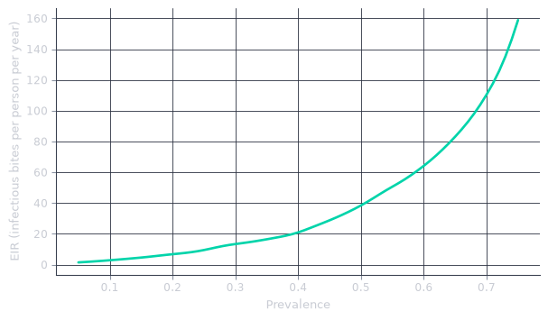
The teal curve is nearly flat below a prevalence of 0.3 and climbs almost vertically above 0.6. Prevalence saturates while transmission does not, so once most of the population carries parasites, a further rise in prevalence can only come from a very large rise in the bites behind it. An input a few points out at 70% therefore moves the inferred EIR by tens of bites per year. The same error at 20% moves it by less than one.
The same measured prevalence implies different EIRs in different settings. Net coverage is the covariate that moves the answer most. Only the coverage varies below.
from estimint import calculate_dn0

rows = []
for coverage in [0.0, 0.3, 0.5, 0.7, 0.9]:
    nets = calculate_dn0(0.30, py_only=coverage)
    rows.append({
        "coverage": coverage,
        "dn0_use": nets.dn0,
        "itn_use": nets.itn_use,
        "Q0": 0.85, "phi_bednets": 0.80, "seasonal": 0.0, "irs_use": 0.0,
        "prevalence": 0.45,
    })

nets_vs_eir = pd.DataFrame(rows)
nets_vs_eir["eir"] = run_xgb_model(nets_vs_eir, prev_model)

nets_vs_eir[["coverage", "dn0_use", "itn_use", "prevalence", "eir"]].round(3)| coverage | dn0_use | itn_use | prevalence | eir | |
|---|---|---|---|---|---|
| 0 | 0.0 | 0.000 | 0.0 | 0.45 | 22.536 |
| 1 | 0.3 | 0.311 | 0.3 | 0.45 | 24.170 |
| 2 | 0.5 | 0.311 | 0.5 | 0.45 | 26.461 |
| 3 | 0.7 | 0.311 | 0.7 | 0.45 | 31.960 |
| 4 | 0.9 | 0.311 | 0.9 | 0.45 | 37.058 |
Every row reports the same prevalence, and the inferred EIR still rises by roughly two thirds down the column, because a district that holds 45% prevalence under 90% net coverage must be absorbing far more infectious bites than one that holds it with no nets. Understating itn_use therefore biases the EIR downwards. Please see Nets and dn0 for that error.
irs_use acts the same way and far more strongly.
irs = pd.DataFrame(
    [{"dn0_use": 0.40, "Q0": 0.85, "phi_bednets": 0.80, "seasonal": 0.0,
      "itn_use": 0.50, "irs_use": v, "prevalence": 0.30} for v in [0.0, 0.2, 0.4, 0.6, 0.8]]
)
irs["eir"] = run_xgb_model(irs, prev_model)
irs[["irs_use", "prevalence", "eir"]].round(2)| irs_use | prevalence | eir | |
|---|---|---|---|
| 0 | 0.0 | 0.3 | 12.13 |
| 1 | 0.2 | 0.3 | 25.34 |
| 2 | 0.4 | 0.3 | 47.53 |
| 3 | 0.6 | 0.3 | 104.70 |
| 4 | 0.8 | 0.3 | 204.43 |
Holding prevalence fixed, the inferred EIR climbs steeply with irs_use, from about 12 with no spraying to about 200 at 80% coverage. Indoor spraying suppresses transmission hard, so a setting that still shows 30% prevalence under heavy IRS is read as one with a very high underlying EIR.
The estimate is only as good as the irs_use you supply, and a value that is too high, or a scenario that pairs a high prevalence with heavy spraying, pushes the EIR into the top of the training range or past it, where it is then clamped. Check the estimated EIR before trusting a trajectory built on it.
set_global_model registers a model as the default, after which run_xgb_model may be called with the frame alone, and get_global_model returns whatever is currently registered.
from estimint import set_global_model, get_global_model

set_global_model(prev_model)
run_xgb_model(one)array([13.39696895])get_global_model()["class"]'estiMINT_model'Note that the global slot holds exactly one model, so pass the model explicitly in any script that touches more than one of the three, because a stray set_global_model elsewhere changes what an unqualified call resolves to.
prev_y9 is clamped to [0.005, 0.80], and values outside that band are pulled to the nearest edge. No warning is raised.
edges = pd.DataFrame(
    [{**setting, "prevalence": p} for p in [0.001, 0.005, 0.80, 0.95]]
)
edges["eir"] = run_xgb_model(edges, prev_model)

edges[["prevalence", "eir"]].round(3)| prevalence | eir | |
|---|---|---|
| 0 | 0.001 | 0.894 |
| 1 | 0.005 | 0.894 |
| 2 | 0.800 | 234.882 |
| 3 | 0.950 | 234.882 |
A sweep producing an implausibly flat EIR at either end has almost always hit this clamp.
Please see EIR and HBR for the same inversion run from entomological data in both directions, and Mosquito density and EIR for the EIR when the vector population changes.