estimate_eir_with_mosquito_delta covers changes that act on the size of the mosquito population rather than through the nets, such as larviciding or a new irrigation scheme, taking a prevalence, a setting and a fractional change in density and returning the EIR that follows. That is an equilibrium value, not a trajectory.
inputs carries one row per scenario and eight columns, prevalence, mosquito_delta, and the six setting covariates dn0_use, Q0, phi_bednets, seasonal, itn_use and irs_use. models is keyword-only. It must hold all three models, under the keys "prevalence", "hbr" and "eir_to_hbr".
mosquito_delta is a fraction rather than a multiplier, so 0.25 is a 25% increase, -0.5 a halving and 0.0 no change. It must be greater than -1.
A note on the older signature
estiMINT 1.4 accepted loose keyword arguments such as prevalence=... and dn0_use=..., one call per scenario, and loaded the models itself. That form has been removed. The current call takes a DataFrame and an explicit models dict, and it is vectorised, so pass every scenario as a row of one frame.
The ratio method
The method runs in five steps, each justified in EIR and HBR.
The prevalence and the setting give a baseline EIR, via the prevalence model.
That EIR and the setting give a baseline HBR, via eir_to_hbr.
The new HBR is the baseline scaled by the density change, hbr_new = hbr_baseline * (1 + mosquito_delta). Density enters here, and only here.
The hbr model predicts an EIR at both HBR values.
The new EIR is the baseline EIR times the ratio of those two predictions.
The EIR the hbr model predicts at hbr_new is not itself the answer, because every prediction from that model inherits the bias measured in EIR and HBR, where an EIR of 13.40 comes back as 14.23. Taking a ratio cancels it.
eir_baseline is identical down the column, because only the mosquitoes changed.
The EIR multiplier
import numpy as npgrid = pd.DataFrame([ {"prevalence": 0.30, "mosquito_delta": d, **setting}for d in np.linspace(-0.75, 1.0, 36)])curve = estimate_eir_with_mosquito_delta(grid, models=models)fig, ax = plt.subplots()ax.plot(grid["mosquito_delta"], curve["eir_multiplier"], label="EIR multiplier")ax.plot(grid["mosquito_delta"], 1+ grid["mosquito_delta"], ls="--", label="proportional response")ax.axhline(1.0, color="#8b93a3", ls="--", lw=1, alpha=0.7)ax.set_xlabel("Mosquito density change (mosquito_delta)")ax.set_ylabel("EIR multiplier")ax.legend()plt.show()
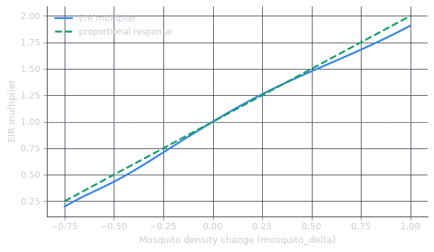
EIR multiplier against fractional change in mosquito density, compared with a proportional response.
The blue multiplier curve sits on the dashed green proportional line for modest changes either side of zero, and within about 10% a proportional response is accurate to a percent or so. At both extremes the blue curve drops below the green one, because deep cuts take the EIR down faster than they take the mosquitoes, so removing three quarters of them leaves about a fifth of the baseline EIR rather than a quarter. Doubling the vectors falls short of doubling transmission.
A note on the input mode
mosquito_delta is honoured when the driving input is a prevalence. In the scenario API of Running scenarios, where the input mode is chosen through EirTarget(value, input_mode), a non-zero mosquito_delta is ignored for input_mode="eir" and input_mode="hbr". No warning is raised, no error is thrown, and the EIR comes back unchanged. The ratio needs a baseline EIR that is independent of the HBR models, and only a prevalence input supplies one. To apply a density change to an EIR or an HBR you already have, scale the HBR yourself and convert.
See also
estiMINT API sets out every loader, estimator and dataclass the package exposes, and Running scenarios carries mosquito_delta through a whole scenario, from the density change to the case counts.