Interventions and nets

MINTverse models three vector-control levers, insecticide-treated nets (ITNs), indoor residual spraying (IRS), and larval source management (LSM).

Net types

ITNs are grouped into four formulations whose names are the keyword arguments to calculate_dn0 and Scenario. They are the allowed values of net_type_future.

Name	Formulation	What it adds
`py_only`	Pyrethroid only	The baseline net
`py_pbo`	Pyrethroid with PBO	Restores kill in resistant populations
`py_pyrrole`	Pyrethroid with a pyrrole (chlorfenapyr)	Kill that does not decay with pyrethroid resistance
`py_ppf`	Pyrethroid with pyriproxyfen (PPF)	An effect on the next generation, folded into `lsm`

net_types() returns the long forms alphabetically, which puts ppf before pyrrole, so indexing into the list rather than naming the net is a common source of error.

import numpy as np
import pandas as pd
from estimint import calculate_dn0, net_types

net_types()

['pyrethroid_only', 'pyrethroid_pbo', 'pyrethroid_ppf', 'pyrethroid_pyrrole']

Short aliases are accepted everywhere the long forms are.

Present and future

Every intervention enters the emulator twice, once for the state of the district before the campaign and once for the state from the campaign onwards. Nets carry a dn0_use and an itn_use for the nets already in the field, and a dn0_future and an itn_future for the nets the campaign distributes. IRS carries irs_use and irs_future the same way. The campaign lands at day 3285, and the present values hold up to it while the future values hold after it.

The two do not have to match, which is what a campaign is. You can keep the same product at the same coverage by restating it, switch pyrethroid-only nets to PBO or pyrrole, raise or lower the coverage, add spraying or larviciding that was not there before, or withdraw the nets by leaving the future fields unset. stateMINT sees the change at day 3285 and nowhere earlier, so the three years before the campaign are identical for any two scenarios that share a present and differ only in the campaign.

Note that the future fields do not inherit the present. Leaving itn_future at zero, or net_type_future at None, models the nets being withdrawn rather than held, which is set out in Covariates and the time grid.

Net effectiveness and dn0

dn0 is the probability that a mosquito is killed when it contacts a treated net, and it depends on the insecticide and on the local level of pyrethroid resistance. calculate_dn0 turns a net mix and a resistance level into that number, and into the total coverage itn_use, which is worked through in Nets and dn0.

Resistance response

Usage is set to 1.0 for one net type at a time.

nets = ["py_only", "py_pbo", "py_pyrrole", "py_ppf"]
resistance = np.linspace(0.0, 1.0, 41)

dn0 = pd.DataFrame(index=pd.Index(resistance, name="resistance"))
for net in nets:
    dn0[net] = [calculate_dn0(r, **{net: 1.0}).dn0 for r in resistance]

dn0.loc[[0.0, 0.25, 0.5, 0.75, 1.0]].round(4)

	py_only	py_pbo	py_pyrrole	py_ppf
resistance
0.00	0.3376	0.5094	0.5611	0.4111
0.25	0.3163	0.4893	0.5526	0.3980
0.50	0.2850	0.4567	0.5371	0.3777
0.75	0.2344	0.3916	0.4964	0.3394
1.00	0.0000	0.0714	0.1522	0.1085

fig, ax = plt.subplots()

for net in nets:
    ax.plot(dn0.index, dn0[net], label=net)

ax.set_xlabel("Pyrethroid resistance")
ax.set_ylabel("dn0 (probability of death on contact)")
ax.set_xlim(0, 1)
ax.set_ylim(0, None)
ax.legend()
plt.show()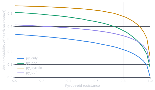

Four declining curves of dn0 against resistance from 0 to 1. The amber pyrrole curve is highest throughout, starting near 0.56 and staying flattest before falling away past 0.75. The green PBO curve starts near 0.51 and the purple PPF curve near 0.41, and the two converge at high resistance and cross at about 0.92, after which purple is the higher. The blue pyrethroid-only curve is lowest throughout, starting near 0.34 and falling to zero at full resistance. — Probability a mosquito dies on contact with a net (`dn0`), against pyrethroid resistance, for each net type at full usage.

The amber pyrrole curve sits above the other three at every resistance level and the blue pyrethroid-only curve below them all, and the ratio between the two grows from about 1.7 at zero resistance to about 2.5 at 0.9. Chlorfenapyr kills through a pathway that pyrethroid resistance does not act on, so the amber curve gives up only the pyrethroid share of its lethality. The blue curve has nothing else to give up. It reaches zero when resistance is total.

The green PBO curve and the purple PPF curve cross at about 0.92. Green runs above purple everywhere below that. PBO works by restoring the kill of the pyrethroid itself, and there is nothing left to restore once resistance is near total, while PPF carries a component that survives it.

The resistance-to-dn0 curves come from the same published source that malariasimulation uses. They are a lookup table, not a fitted model.

IRS and LSM

IRS and LSM enter as coverage proportions, where irs_use is the spraying coverage in place now, irs_future the coverage under the campaign being evaluated, and lsm the larval term. All three are on a 0 to 1 scale. Neither IRS nor LSM has a dn0-style effectiveness term.

run_scenarios folds PPF coverage into lsm before the emulator runs, at a factor of 0.248. The factor is not configurable.

\[ \texttt{lsm\_eff} = \min\big(\texttt{py\_ppf} \times 0.248 + \texttt{lsm},\ 1.0\big) \]

PPF nets at 0.5 coverage and LSM at 0.30 reach the emulator as \(0.5 \times 0.248 + 0.30 = 0.424\).

The lsm column is lsm_eff

The lsm column in the run_scenarios output is reported after the PPF contribution has been added, so it is not the lsm you passed. It is the column that will not match when you reconcile a scenario’s inputs against its outputs.

Limitations of dn0

dn0 summarises the probability of death on contact, and nothing else. Repellence is not in it.

Nor does it capture attrition, since dn0 and itn_use are held constant across the trajectory, so a campaign’s protection arrives in full at day 3285 and holds.

A single mix covers the whole population, so a district where half the villages have new nets and half have five-year-old nets is represented as one uniformly in the middle.

A setting above 0.75 resistance sits in the steep part of every curve, where a small error in the resistance level supplied produces a large error in dn0, so vary it in a sensitivity check rather than trusting a single value.