The columns of a (B, 157) array are fortnightly windows spanning six years of simulation. Plot against time relative to the campaign. The campaign then sits at zero.
The setting
The running example is a district with a measured under-5 prevalence of 0.45. Pyrethroid resistance is 0.30 and pyrethroid-only nets are at 70% coverage.
The three candidate campaigns below are all at 70% coverage and differ only in the net product, and each restates itn_future. Leaving it at zero would withdraw the nets.
fig, (ax_p, ax_c) = plt.subplots(2, 1, figsize=(7.2, 6.4), sharex=True)for label, p, c inzip(products, prev, case): ax_p.plot(years, p, label=label) ax_c.plot(years, c, label=label)for ax in (ax_p, ax_c): ax.axvline(0, color="#8b93a3", ls="--", lw=1, alpha=0.7)ax_p.set_ylabel("Prevalence")ax_p.set_title("Parasite prevalence")ax_p.legend(loc="lower right")ax_c.set_ylabel("Cases per 14-day window")ax_c.set_xlabel("Years relative to the campaign")ax_c.set_title("Clinical cases")plt.show()
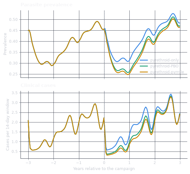
Prevalence and clinical cases under three net products, all at 70% coverage, in a district with pyrethroid resistance of 0.30. Blue is pyrethroid-only, green is PBO and amber is pyrrole. The dashed rule marks the campaign.
Interpreting the figure
The blue, green and amber curves lie on top of one another to the left of the dashed rule. They separate only to the right of it. The campaign covariates are masked before day 3285. Curves separating before the rule mean something in the present has changed, most often dn0_use, itn_use or the EIR.
That shared baseline is not flat, because model_start_day is day 2190 and the campaign is day 3285, one three-year mass-distribution cycle apart. The window opens on the previous distribution and closes on the next. Prevalence falls through the first year as those nets take effect. It climbs for two more as they wear out and are not replaced.
pre = prev[:, :idx_y9 +1]annual = {}for a inrange(-3, 3): in_year = (years >= a) & (years < a +1) annual[a] =float(prev[0][in_year].mean())print("prevalence given to estiMINT :", 0.45)print(f"emulator at the campaign : {prev[0, idx_y9]:.3f}")print()print(f"pre-campaign range : {pre.min():.3f} to {pre.max():.3f}")print(f"campaigns identical before 0 : {bool(np.allclose(pre[0], pre[1]) and np.allclose(pre[1], pre[2]))}")print()for a, mean in annual.items():print(f"mean prevalence, year {a:+d} : {mean:.3f}")
prevalence given to estiMINT : 0.45
emulator at the campaign     : 0.456

pre-campaign range           : 0.288 to 0.491
campaigns identical before 0 : True

mean prevalence, year -3   : 0.332
mean prevalence, year -2   : 0.369
mean prevalence, year -1   : 0.455
mean prevalence, year +0   : 0.339
mean prevalence, year +1   : 0.402
mean prevalence, year +2   : 0.490
The three campaigns are identical before the rule, and at the campaign step the trajectory passes within a few thousandths of 0.45, the prevalence estiMINT was given. Run that check on every scenario.
The agreement holds at idx_y9 and not on average, because the annual means run from 0.33 to 0.46, and a trajectory that misses the measured prevalence at idx_y9 means something is wrong upstream, most often in dn0_use or itn_use.
Three years on, the curves are ordered as the dn0 table predicts, with amber pyrrole lowest, green PBO above it, and blue pyrethroid-only highest in both panels, and they differ only in dn0_future, so at 30% resistance the pyrrole net kills the largest share of the mosquitoes that touch it.
A tidy frame
A groupby or a CSV for a collaborator wants the data long, one row per scenario per timestep.
frames = []for i, net inenumerate(products): frames.append(pd.DataFrame({"net": net,"years": years,"abs_day": abs_t,"prevalence": prev[i].astype(float),"cases": case[i].astype(float), }))tidy = pd.concat(frames, ignore_index=True)print(tidy.shape)tidy.head()
(471, 5)
net
years
abs_day
prevalence
cases
0
pyrethroid-only
-3.000000
2190
0.449371
2.086377
1
pyrethroid-only
-2.961644
2204
0.450827
1.185663
2
pyrethroid-only
-2.923288
2218
0.438303
0.658037
3
pyrethroid-only
-2.884932
2232
0.415712
0.613480
4
pyrethroid-only
-2.846575
2246
0.393178
0.564645
Each net contributes a block of 157 rows, and pd.concat stacks the three. The astype(float) widens the emulator’s float32 output to double, which stops rounding from producing things like 274.299988. tidy.to_csv("trajectories.csv", index=False) writes a file anyone can open in R.
post = tidy[tidy["years"] >=0]post.groupby("net", sort=False)["cases"].sum().round(1)
Summing over all 157 windows adds the same three baseline years to every product. Cases averted and relative reduction therefore both come out understated. Filter to years >= 0 before totalling anything.