A Scenario describes one setting and one campaign, and run_scenarios takes a list of them and returns a table with one row each. Both are dataclasses, importable from estimint or estimint.scenarios.
from estimint import run_scenariosfrom estimint.scenarios import Scenario, EirTarget
The seven required fields
These have no defaults and must always be given.
Field
Meaning
name
A label. It is echoed into the results and is how you index them afterwards.
res_use
Pyrethroid resistance, 0 (fully susceptible) to 1 (fully resistant).
Q0
Human blood index, 0 to 1.
phi
Share of bites taken while people are in bed. Enters the emulator as phi_bednets.
seasonal
0 for perennial transmission, 1 for strongly seasonal.
irs
IRS coverage currently in place. Enters the emulator as irs_use.
eir_target
An EirTarget. How transmission intensity is specified.
res_use is not a covariate, and is consumed by the dn0 curves without reaching the emulator. What it sees is the twelve static covariates.
The input modes
EirTarget(input_value, input_mode) says what quantity you are handing over, and because the emulator only ever runs from an EIR, the mode decides what has to happen first. Almost always the value is a measured prevalence.
Mode
You supply
What happens
"prevalence"
Under-5 parasite prevalence in [0.005, 0.80]
estiMINT inverts it to an EIR with the XGBoost prevalence model.
"eir"
An EIR, infectious bites per person per year
Used directly. No inversion.
Use "prevalence" for a cross-sectional survey and "eir" when the EIR is in hand or is being swept over. A third mode, "hbr", takes a human biting rate, but the HBR is a quantity the pipeline works out rather than one a programme measures, so it is rarely supplied directly.
Note that mosquito_delta only applies to "prevalence", and supplied alongside an "eir" or an "hbr" input it is ignored. The mechanism is set out in Mosquito density and EIR.
The ten defaulted fields
Everything else defaults to zero or None.
Field
Default
Meaning
py_only
0.0
Current coverage of pyrethroid-only nets.
py_pbo
0.0
Current coverage of pyrethroid-PBO nets.
py_pyrrole
0.0
Current coverage of pyrethroid-pyrrole nets.
py_ppf
0.0
Current coverage of pyrethroid-PPF nets.
mosquito_delta
0.0
Proportional change in mosquito density. Must be > −1.
itn_future
0.0
Net coverage from the campaign.
net_type_future
None
Net product from the campaign.
irs_future
0.0
IRS coverage from the campaign.
routine
0.0
Routine (continuous) net distribution from the campaign.
lsm
0.0
Larval source management coverage from the campaign.
The first four are the current net mix, whose coverages are summed to give itn_use and whose dn0 values are averaged to give dn0_use. routine and lsm carry no _future suffix but belong to the campaign all the same, and like dn0_future, itn_future and irs_future, they are held at zero before day 3285 and take their supplied value only from the campaign onwards.
Future coverage must be set explicitly
If itn_future is 0 or net_type_future is None, then dn0_future and itn_future are both set to 0 and the nets are withdrawn at the campaign. irs_future behaves the same way and does not inherit from irs.
To hold an intervention steady you have to restate it. A setting with pyrethroid-only nets at 0.70 coverage that keeps them needs itn_future=0.70, net_type_future="pyrethroid_only" written out in full. Omit it and the nets have been modelled as abandoned.
Five scenarios
The five scenarios below vary every axis the pipeline exposes, and are five different settings rather than five campaigns in one. There is no shared baseline.
import numpy as npimport pandas as pdfrom estimint import run_scenariosfrom estimint.scenarios import Scenario, EirTargetscenarios = [# A prevalence survey, pyrethroid-only nets held at their current coverage. Scenario(name="Pyrethroid-only, prevalence", res_use=0.30, Q0=0.85, phi=0.80, seasonal=0.0, irs=0.0, eir_target=EirTarget(0.45, "prevalence"), py_only=0.70, itn_future=0.70, net_type_future="pyrethroid_only"),# A seasonal setting under PBO nets and IRS, with mosquito density rising 60%. Scenario(name="PBO, +60% mosquitoes", res_use=0.55, Q0=0.90, phi=0.85, seasonal=1.0, irs=0.40, eir_target=EirTarget(0.30, "prevalence"), py_pbo=0.85, mosquito_delta=0.60, itn_future=0.85, net_type_future="pyrethroid_pbo", irs_future=0.40),# Pyrrole nets plus larviciding, with mosquito density halved. Scenario(name="Pyrrole + LSM, -50% mosquitoes", res_use=0.70, Q0=0.75, phi=0.70, seasonal=0.0, irs=0.0, eir_target=EirTarget(0.30, "prevalence"), py_pyrrole=0.60, mosquito_delta=-0.50, itn_future=0.60, net_type_future="pyrethroid_pyrrole", lsm=0.30),# A prevalence survey with PPF nets, whose coverage folds into effective larviciding. Scenario(name="PPF, prevalence", res_use=0.45, Q0=0.80, phi=0.82, seasonal=0.0, irs=0.0, eir_target=EirTarget(0.35, "prevalence"), py_ppf=0.50, itn_future=0.50, net_type_future="pyrethroid_ppf"),# The EIR is already known, so estiMINT does nothing. IRS only, no nets at all. Scenario(name="No nets, EIR given", res_use=0.0, Q0=0.88, phi=0.78, seasonal=1.0, irs=0.60, eir_target=EirTarget(20.0, "eir"), irs_future=0.60),]res = run_scenarios(scenarios)res.shape
(5, 23)
run_scenarios resolves each scenario, then assembles the twelve covariates and calls the emulator once with the whole batch.
Net type names
net_type_future accepts "pyrethroid_pbo" or the short alias "py_pbo". It does not accept "pyrethroid-pbo". A hyphen raises ValueError: unknown net type.
The returned columns
The columns fall into four groups, of which the first is what you asked for, resolved, with the current net mix reduced to a single product name.
res[["name", "input_mode", "net", "net_future"]]
name
input_mode
net
net_future
0
Pyrethroid-only, prevalence
prevalence
py_only
pyrethroid_only
1
PBO, +60% mosquitoes
prevalence
py_pbo
pyrethroid_pbo
2
Pyrrole + LSM, -50% mosquitoes
prevalence
py_pyrrole
pyrethroid_pyrrole
3
PPF, prevalence
prevalence
py_ppf
pyrethroid_ppf
4
No nets, EIR given
eir
none
none
With no campaign nets, net_future comes back as the string "none" rather than as a missing value.
The second group is the covariates the emulator actually saw, derived rather than echoed back.
dn0_future is the campaign product’s dn0 at that resistance.
Note that lsm is not always the lsm you passed, since run_scenarios folds PPF net coverage into effective larval source management, under the rule set out in Interventions and nets. The fourth row passed none and comes back with one.
The third group is transmission intensity, where eir_baseline is what the inversion produced and eir_final is that EIR after mosquito_delta has been applied. The two are equal whenever the delta is zero.
In the second row a 60% rise in mosquito density roughly doubles the EIR, while in the third, halving the density cuts the EIR by more than half. Neither response is proportional to the change.
hbr_baseline and hbr_new are populated only for those two rows, since the HBR is an intermediate in the mosquito-density calculation. They are NaN everywhere else.
The fourth group is outcomes, where prev_y9 is prevalence at the campaign and a scenario that supplied a prevalence should recover it closely.
The second and third rows both supplied 0.30 and recover 0.261 and 0.198, and the third is well off, deliberately so, because a mosquito-density adjustment of −50% moves the EIR away from the one that sustained the measured prevalence.
prev_endline and cases_endline are the horizon’s last window, three years on.
The trajectories
The last two columns, prevalence and cases, are not scalars. Each cell holds the full trajectory as a 157-element NumPy array.
The frame cannot be written to CSV, and any comparison across scenarios has to reach into the cells first. Exporting results deals with both.
The 157 windows are a property of the emulator, so read the grid off the artefact rather than hard-coding it. preload_models returns the three estiMINT XGBoost models and the two stateMINT artefacts. Calling it once up front fills the caches and pulls the weights from Hugging Face before the first run.
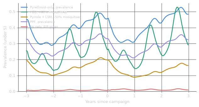
Prevalence under all five scenarios. The dashed line marks the campaign at year 0, and everything to its left is the run-up under whatever was already in place.
The five lines start at different levels, and the three years to the left of the grey dashed line are each model’s run-up to its campaign. The prevalence you supply is therefore prevalence at the campaign, not at the start of the horizon. The value to check it against is prev_y9.
The weights repository
Both run_scenarios and preload_models take an hf_repo argument, defaulting to "dide-ic/stateMINT".
res = run_scenarios(scenarios, hf_repo="dide-ic/stateMINT")
Change it to run against a fork or a local snapshot. Note that run_scenarios tracks whatever main points at in that repository and exposes no revision pin. For a reproducible analysis, record the weight version alongside the results, or drive the emulator directly with a pinned revision as in Calling the emulator.